

The RATE function in Excel belongs to the group of financial functions commonly used in financial mathematics and interest rate calculations or/and in finance analysis. Along with several other functions, it is typically used to determine the parameters of a loan.
In the previous article, we explained how to use the NPER function and demonstrated that it allows us to calculate the number of payment periods required to repay a loan, given the following parameters:
- annuity payment (PMT function)
- interest rate
- loan amount
In this article, we will show how to calculate the interest rate using the RATE function, provided that we know:
- the annuity payment,
- the loan amount, and
- the number of periods.
Syntax of the RATE Function in Excel
=RATE( nper; pmt; pv; [fv]; [type] )

Example: Using the RATE Function
Similar to the previous article about the NPER function, we will use the same example from the article PMT – Loan Payment and Amortization Schedule, where we calculated the amount of the annuity payment.
Let’s recall the parameters of that example — we were calculating the payment for a loan with the following details:
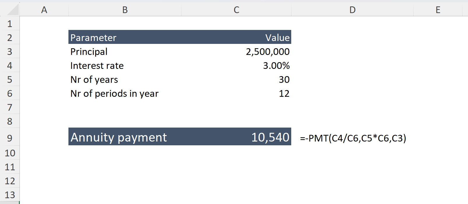
After performing the calculation, the payment amount was 10,540 USD
In the previous article, we confirmed that all Excel financial functions are interconnected. We also demonstrated that by using the NPER function together with parameters such as payment amount (calculated using PMT), interest rate, and loan principal, we can determine that the loan term is exactly 30 years.
Now, let’s verify whether we can arrive at an interest rate of 3% using the RATE function, given the following parameters:
- annuity payment = 10,540 USD
- loan amount = 2,500,000 USD
- number of periods = 30
Important note: An annuity payment is almost always calculated on a monthly basis. Therefore, the number of periods must be entered in months, and the resulting monthly interest rate must be multiplied by 12 to obtain the annual rate (since the function returns a monthly rate).
